In the previous posts Feasibility is optimal and On self-concordant convergence I have made the case that seeking centrality may be better than trying to optimize on some objective function. The reason for this is two-fold:
- there is uncertainty in the data that make up the constraints
- seeking centrality gives each workplace more leeway
In this post I will go into the second point, describing how we might quantify the amount of leeway/autonomy that can be provided to each workplace "no questions asked" by the system as a whole.
Defining workplace autonomy
What I mean by autonomy in this post is the extent to which each workplace can govern itself without threatening the feasibility of the system as a whole. The less constrained each workplace is the more "free" the workers in that workplace are likely to be. The more orthogonal its actions can be to the rest of the economy, the freeër it is. But at the same time, no workplace is an island.
Excessive production of some products may induce demand or side-effects in other parts in the system that exceed the system's capabilities, thus violating feasibility. Greenhouse gas emissions are the obvious example, but other issues like eutrophication are also a concern, as happens currently with the southern parts of the Baltic sea (Övergödning och läckage av växtnäring, Eutrophication and leakage of plant fertilizer, Jordbruksverket, fetched 2023-05-15). Likewise insufficient production will cause shortages in downstream workplaces, also violating feasibility.
A maker of electric motors may speculatively try to make products in excess of the supply of rare-earth elements for magnets, which obviously will cause shortages in other parts of the economy, and thus such production should be discouraged. But if they don't exceed said supply, then it may be worthwhile to produce more than is currently demanded because tooling costs amortize. This would lower the cost of the products overall, and allow the workers there to take time off. Therefore for work scheduling purposes it would be useful to know within what bounds production can be guaranteed to proceed smoothly, assuming sufficiently accurate data in the relevant parts of the system. The more orthogonal a workplace is to the rest of the economy, the easier the scheduling of its work becomes.
Being able to answer these questions by machine quickly means less bureaucracy, also an obvious boon to workplace autonomy.
Finally, when workers in a workplace know that they can reduce production by a certain amount for a certain length of time, this allows exploring other production methods. For example another type of plant can be planted or another gizmo invented using the resources so freed up. We can imagine many remuneration schemes encouraging such exploration. There is always a tradeoff between exploration and exploitation, a problem known as the multi-armed bandit.
The geometry of workplace autonomy
I have mentioned orthogonality above. In this section I will show what this means.
Let us for simplicity in visualization imagine two workplaces, A and B. A makes product a and B makes product b. It is estimated by both workplaces independently that for some time period A can produce between 0-100 units of a and B can produce 0-50 units of b. Each unit of a and b produces one unit of emissions, and the total amount of emissions are to be kept below 110. The estimated demand for a is 40 and the estimated demand for b is 10. Let us assume that the center of the system is at , . The situation looks like the following figure:

The diagonal line corresponds to the emissions constraint. It may be tempting for each workplace to look at this and derive updated bounds on their own production without taking the other into consideration, namely and :

However as sharp-eyed readers may realize, if both workplaces act entirely autonomously using only these bounds as reference then feasibility cannot be guaranteed. The Cartesian product of the two bounds is a rectangle, part of which lies outside of the feasible region:

The orthogonality I have mentioned is here apparent. The rectangle's sides are orthogonal (at 90°) to one another.
There are many choices for feasible rectangles in this system, and the most straightforward one seems to be to scale the limits on both a and b down so that the upper-right corner of the rectangle lies on the emissions constraint, like so:

The updated bounds are and . Many other feasible bounds are possible. This approach generalizes to any number of workplaces and production methods, meaning we can always fit some n-dimensional rectangle (orthotope or box) inside the system. All that is necessary is that all corners of the box lie within the feasible region.
Other geometries are also possible. Production within one workplace having two production methods available could be limited not just to a rectangle but any convex polygon, for example a hexagon. The Cartesian product of such a polygon with another workplace having just one production method results in a prism.

Note that the sides of the prism are orthogonal to its ends. This orthogonality is again key to why autonomy can be guaranteed. That the edges of the hexagons are not orthogonal to one another is here a strength, since this allows more autonomy within the associated workplace. We can quantify the degree of autonomy by the area of the hexagon. For the other workplace it is the length of the sides between the two hexagons. For the system as a whole the total autonomy is the volume of the prism, which is just the product of the hexagon's area and the side length.
If the number of production methods is larger than three then the result is a prismatic polytope, which are difficult to illustrate for obvious reasons. Such polytopes have properties that make them easier to deal with computationally than polytopes in general.
Note that two or more workplaces coordinating their actions more tightly can get a combined larger volume to work within, at the cost of reduced autonomy and at the cost of more infernal meetings. The figure below illustrates a situation where the heaxgonal workplace has more room to work within when the linear workplace is closer to the "lower" state. The resulting shape is a frustrum.

It should hopefully be clear that the two workplaces are now dependent on more communication than before. Note that the amount of necessary communication can be attenuated by an automatic plan solver. But the roundtrip time inherent in that may be irritating to workplace coordination, for example when assigning shifts. Hence a preference to autonomy.
A small demo
Apologies to those who are even more averse to JavaScript than I am, but I know of no way to do the following using just HTML+CSS.
The system below is the same as the one before. Try dragging the slider and see what happens. The dot doesn't move, sorry. Patch welcome!
A more complicated example would use multiple workplaces with multiple production methods and a simulated delay, showing how two or more workplaces stepping outside the box can result in infeasibility that isn't immediately visible. Perhaps something for the future..
A fast box fitting algorithm
Consider the closed polytope with and a non-zero internal volume, and some internal point around which we'd like to find a large n-dimensional box . Without loss of generality we can change the coordinate system to make the origin correspond to . The updated system is where all entries in by necessity are negative. If we want we can again without loss of generality scale each row in so that all entries in are -1. The implementation does this, but for clarity the description does not.
Next introduce the positive vectors and , the lower and upper bounds that make up , like so:

The corners of have the coordinates and because and the origin is always contained in the box. It is easy to see that the (hyper)volume of the box is
We would ideally like to compute the largest feasible box that contains the origin, or if we can't guarantee optimality then we at least want a box that is not unreasonably small. The algorithm proposed here is one that produces a reasonable, but not necessarily optimal, .
We start by observing that for all rows there is a set of corners that minimize the scalar product with . In other words the corners that violates the constraint the most, or if they don't violate it then they are the least slack. These corners have signs opposite of . Dimensions corresponding to zeros in are irrelevant. We can therefore describe the entire set of corners by with signs opposite of , including zeros (which are set to zero in ), like so:
If violates the constraint then we have
with both sides of the inequality negative. We can easily compute a that turns this violated inequality into an equality:
Therefore diminishing the elements in and corresponding to the positive and negative elements in respectively, by multiplying them by , results in a new that is feasible and as a result all other corners in are also feasible with respect to . This because for entries corresponding to non-zeroes in flipping the sign always results in a scalar product that is greater than , that is they are more slack. Note that the diminishing of any entry in or moves entire sets of corners because is parametrized in terms of these two vectors. The corners move as a result of modifying the constraints that make up .
The above implies that no feasible corner can ever be made infeasible by diminishing any of its corresponding elements in and . The new box is always contained within the old box. In the extreme we can diminish and so they are arbitrarily close to the origin, and we can always find some finite and that will fit the bill because the origin is strictly feasible by definition () and so we can always squeeze and into the gap. In fact this algorithm is motivated partly by improving the lower bound on the volume of . We can always compute a box that will fit by first fitting an orthoplex, or more specifically a type of asymmetric lozenge, by tracing in the positive and negative cardinal directions, resulting in initial values for and .
To make the above less abstract let's look at some figures. Let's start with a polygon with the origin in its interior:

By tracing in the cardinal directions we can fit a lozenge within it, which is guaranteed to always work because the polygon is convex:

Finding the rectangle that is the dual to this lozenge (blue) is easy, as is finding the rectangle to which the lozenge itself is the dual (red):

In general the lozenge has the following hypervolume:
The smaller box provides a lower bound on the volume of the large box we seek:
The larger box naturally provides the upper bound:
Obviously is a rather large range, so the chances of us finding a box that is not so horrible are probably good. Keeping in mind that , the bound is equivalent to say a cobbler having leeway to make anywhere between 9.999999999 and 10.000000001 shoes in a given period. Not hooray. So the point is to widen these bounds to something more reasonable, perhaps 5 to 15 shoes.
We are now ready to list the algorithm:
- Compute initial and by tracing lines in the positive and negative cardinal directions from the origin, assigning each entry based on the closest constraint encountered
- For :
- For let
- If
- Let
- For if then update
- For if then update
This results in something like the green rectangle in the figure below:

The complexity of a sparse implementation of the above algorithm is . The basic idea can be modified in various ways, for example permuting the rows in the system so that the algorithm processes them either in increasing or decreasing order of slackness. Another possibility is making multiple passes, using smaller fractions of (say 10%), only using the full in the last pass. Finally the elements in and need not be adjusted by the same but could use some other weighting as long as the result is that the corner is feasible. Formulated as a diagonal matrix , we would then seek:
Paralellizing the algorithm should also be possible, and should work well when there are few off-diagonal elements. Such elements would need to be taken care of in a set of finishing passes.
Because and are very likely not equal, we can recenter the system by adding half their difference to :
I am not sure what the convergence properties are of a method like this, but one useful property is that no linear system solves are required. That makes such a method similar to Katta Murty's most recent work. In case it isn't obvious: after recentering, the above algorithm can be repeated and then the system recentered yet again etc.
A GNU Octave implementation is listed at the end of this post.
Other shapes
The algorithm above is limited to the box geometry and does not play well with for example sum constraints. To make the problem more visible, let's take a farm as an example.
Let us presume that we can plant three types of crops in a region: potatoes, barley and wheat. Because we have a fixed amount of land available, let's say 30 hectares, we might quantify this as:
The algorithm above may output that 5-10 hectares of each of the three crops can be planted without inconveniencing anyone else. This doesn't sound so bad, until one considers what happens if instead 3000 different crops are made available to the solver. After all, why should the choice of crops be limited to only three? In this case the solver would have little choice but to spit out 3000 individual bounds, each one something like "plant 50-100 square meters of this crop". For 3000 crops.
A more reasonable parametrization might be one that outputs a total area to plant, and perhaps minimum amounts of certain crucial crops. Something like "plant 15-30 hectares in total of which at least 5 hectares are potatoes". Geometrically this corresponds to a simplex which has had a smaller simplex subtracted from it. In two dimensions this is a triangle with a smaller triangle taken out:

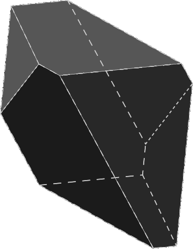
This shape has corners. It would be nice if we could also introduce maximum constraints, but the resulting shape (a truncated simplex) has more than corners in some cases. Compare for example the 8-simplex (9 corners) to the quadritruncated 8-simplex ( corners). This may or may not be a problem, depending on whether the corners that minimize slackness with respect to a given constraint can be found quickly. Perhaps a reader has a solution. If so, let me know! For a box the problem is easy, as demonstrated by the algorithm earlier. The figure below of a truncated tetrahedron with 12 corners drawn using SolveSpace hopefully illustrates the problem:
Moving on, it bears repeating that these shapes represent the bounds within which production can happen with minimal coordination. The necessary inputs will always be provided if staying within it. It might be possible to "color outside the lines", but doing so means a risk of having to go to anywhere between zero and 10,000 meetings. The illustration below might represent a typical situation:

The green area is the same "safe" area as before, but around it is an orange area that will at least require a roundtrip to the planning cloud which may either accept or reject the proposal. It might also be necessary to go to meetings with workplaces both upstream and downstream. Yes dear reader, I hate meetings.
Appendix
GNU Octave implementation of the algorithm.
n = 64;
m = n*100; % the larger the ratio m:n the lower max_k becomes
q = 160;

% generate system
function [A,b,x] = generate(m, n, q)
  m, n, q
  A = sprandn(m, n, min(1,q/m));
  % without loss of generality we can let b be all -1's
  % this makes loz() a bit simpler
  b = -ones(m,1);
  x = zeros(n,1);
endfunction

% compute largest lozenge centered on x
function [l,u] = loz(A, b, x)
  n = size(A,2);
  l = zeros(n,1); % minuses
  u = zeros(n,1); % pluses
  for i = 1:n
    % this can fail for very sparse A because sometimes there are no positives and/or negatives in a column
    % this only works when b is all -1's, I can't be bothered making it prettier because it's not necessary
    l(i) =  1./full(max(A(find(A(:,i)>0),i)));
    u(i) = -1./full(min(A(find(A(:,i)<0),i)));
  endfor
endfunction

function [L,U] = loz2box(A, b, x, l, u)
  [m, n] = size(A);
  for i = 1:m
    % compute several times, checking each pass after the first one
    for p = 1:10
      if p <= 2
        % pick the corner that is most ornery the first two times
        s = full(sign(A(i,:)));
      else
        % pick a random corner in subsequent passes
        s = 2*floor(rand(1,n)*2)-1;
        % the following also picks points on edges, but they are never as nasty
        % s = floor(rand(1,n)*3)-1;
      endif

      l0u = [l,zeros(n,1),u];
      delta = -(l0u((1:n)+(s+1)*n).*s)';
      d = A(i,:)*(x+delta) - b(i);

      if d < -eps*sqrt(n)
        if p > 1
          % this should never happen if we got l and u right
          s, d
          error("d < 0 with p == 2");
        endif
        f = A(i,:)*x - b(i);
        k = 1 + d / (f - d);
        for j = 1:n
          if s(j) == 1
            u(j) *= k;
          elseif s(j) == -1
            l(j) *= k;
          endif
        endfor
      endif
    endfor
  endfor
  L = l;
  U = u;
endfunction

% generate system and compute largest inscribed lozenge at x
[A,b,x] = generate(m, n, q);
[l,u] = loz(A, b, x);

% compute volume of enclosing (max) and enclosed (min) boxes
Vmin = sum(log10((l+u)/n))
Vmax = sum(log10(l+u))
% the lozenge is certainly larger than Vmin but also much smaller than Vmax
Vloz = Vmax - sum(log10(1:n))

% find a large box that is enclosed by Ax >= b
[L,U] = loz2box(A, b, x, l, u);
V = sum(log10(L+U))

if V < Vmin || V > Vmax
  error("bad V");
endif

% compute the maximum and geometric mean k either element were adjusted by
a = [l./L;u./U];
min_k = min(a)
geometric_k = mean(a,"g")
max_k = max(a)
Example output:
octave:1> cube
m = 6400
n = 64
q = 160
Vmin = -123.27
Vmax = -7.6718
Vloz = -96.775
V = -34.632
min_k = 1.1804
geometric_k = 2.7335
max_k = 10.760
What we see here is that the volume of the computed is between Vmax and Vloz. The 's encountered are between 1/1.1804 and 1/10.760 with the geometric mean being 1/2.7335. So the amount of leeway per workplace in the model above is around one third of the naïve min/max bounds computed locally in the lozenge step. What these values are for a real economy would require research. And again, a different geometry that plays more nicely with sum constraints would be desirable.